Systems Applications - Combat Models

Applications of Systems of Differential Equations

Combat Models: Who Will Win The Battle?

Introduction

Another interesting application of systems of differential equations is in the analysis of warfare between two opposing forces. We will consider three possible situations:

1. The Guerilla Combat Model, in which the two opposing armies wage warfare by using guerilla tactics such as sneak raids on the opposition's base or ambush upon each other

2. The Mixed Combat Model, in which a guerilla force is in conflict with an army employing conventional warfare methods

3. The Conventional Combat Model, in which both armies wage war using conventional methods

In creating all three of the models, the general idea behind each model is to create an equation which accounts for the main components which contribute to the rate at which each army is changing. Such issues as the combat effectiveness of the opposing army, the occurrence of accidents, the failure of supply lines, and the rate of reinforcement may all come into play.

Without further ado, let's move on to the first of our analyses...

Guerilla Combat Model

In this situation we suppose that both of the armies involved are waging guerilla warfare on the other. A possible model for the scenario may be the following system of differential equations:

where x(t) represents one guerilla force strength at time t, call them the Xanudian Liberation Front, and y(t) represents the other guerilla force strength at time t, say the Yarovian People's Organization. Furthermore, x_o is the initial Xanudian strength, and y_o is the initial Yarovian strength. Let's suppose that all quantities are in thousands of troops. Carefully consider the relationships of the variables.

In a combat model, x′(t) and y′(t) are called the combat loss rates of the two armies. If you consider the two combat loss rates in the model above, they seem to obey common sense principles. The quantity, x(t) y(t), in both differential equations is a measure of the total number of inter-force encounters possible. The rates are negatively influenced by encounters with the opposing force, since when these forces encounter one another, they attempt to destroy their opponents. It would appear that in the current model the Xanudians are the better fighters, since they inflict a heavier combat loss rate on the Yarovians.

Now for our analysis of the model using Mathematica. I will assume in the following discussion that you have already done the previous two DE-systems-applications labs, and that you are therefore needing less step by step help with the details.

Switch to Mathematica by clicking on the button at left. This will open up a fresh notebook for you. Then return here immediately for further instructions.

1. Let's begin by considering a situation in which both forces have an equal number of troops, say x(0) = 25, y(0) = 25, where both are measured in thousands. Use the NDSolve command, just as you did in the previous two labs, to solve the above system of differential equations, along with the initial conditions just given. Use the interval 0 ≤ t ≤ 30, and read the solution into the variable guerilla1.

2. That shouldn't have taken too long. Now make a phase-plane diagram by using ParametricPlot, just like you did when analysing predator-prey problems in the previous lab. Remember, you'll be plotting {x[t],y[t]}/.guerilla1[[1]] this time, and your t interval is from 0 to 30. Include a PlotRange->All option in your command, and also an AxesOrigin->{0,0} option to force the axes to cross in the location you are used to, and assign the graph to the variable guerillaplot1.

3. Hmm, just about the most boring graph that we've seen in this course. Anyway, now for the important question: Who won?

   Remember that your initial condition was (25, 25). This means that you start your solution (with respect to time) in the top right corner of the graph, and as time passes you move down and to the left along the solution line. You can determine who won by observing where this solution "curve" ended up. It looks like it stops at about (12.5, 0) on my plot. That would be 12,500 Xanudians, and zero Yarovians. I'd say that the Xanudians won! This is in agreement with our initial observation that the Xanudians are better fighters.

   By the way, a couple of remarks: The model ceases to make sense if your solution curve ventures out of the first quadrant. (Why?) And, in general, what does the intersection of the solution curve with an axis (in standard position) mean in the "real world" for this model?

   Well, maybe we should let the Yarovians have more troops to start with. Redo steps 1 and 2 above, but this time with initial conditions x(0) = 25, y(0) = 50. Of course, name your results guerilla2, and guerillaplot2 this time.

4. Who won the battle now? (You should have found that the two forces completely wiped each other out, kind of along the lines of USA/USSR nuclear arms policy during the cold war.) This result probably didn't surprise you. Let's redo steps 1 and 2 again, this time with initial conditions of x(0) = 25, y(0) = 75. In other words we're giving the Yarovian force an even larger army than in the last scenario. Rename your variables guerilla3, and guerillaplot3 this time.

5. At last, the Yarovians score a victory (about 25,000 of their troops survived)! What seems to be the basic requirement for a Yarovian victory in this model? It looks like they have to have more than twice the number of troops as the Xanudians, probably due to the fact that the Xanudians fight twice as effectively.

6. Finally, use the Show command to display all three graphs on the same coordinate system. (Is there any wonder that guerilla vs. guerilla warfare is said to obey the linear combat law?)

OK, that takes care of the guerilla vs. guerilla scenario. Let's move on to a slightly more interesting situation...

Mixed Combat Model

In this model we have a guerilla force fighting against a conventional army. A possible model for this situation might be this system of differential equations:

where g(t) represents the guerilla force strength at time t, and c(t) represents the conventional force strength at time t, g_o is the initial guerilla strength, and c_o is the initial conventional force strength. All numbers are measured in thousands. Once again, carefully consider the relationships of the variables.

This time the combat loss rates of the two forces aren't symmetric with respect to one another. The guerilla combat loss rate is proportional to the number of guerilla-conventional encounters, whereas the conventional combat loss rate is proportional only to the number of guerillas. Think about their differing styles of warfare, and you might see why this should be so. Guerillas don't choose to fight a conventional force openly, but favor tactics such as ambush, and sneak raids on army bases.

1. Solve the mixed combat system above with the initial conditions g(0) = 10, c(0) = 15. Use the interval 0 ≤ t ≤ 10, and read the solution into the variable mixed1. Follow this up with a phase-plane diagram, which you assign the name mixedplot1.

2. So who won this time? It looks like the solutions ends around (0, 5). Since the first coordinate represents guerillas, and the second represents the conventional army, it would appear that the guerillas were all killed, and 5,000 conventional troops survived.

   Redo the problem using each of the following ordered pairs as initial conditions of the form (g_o, c_o): initial conditions (8, 15), (9, 15), (11, 15), (12, 15), (13, 15). Name your solutions and plots appropriately. (Oh, on the last one, stop t at 5 instead of at 10—this will prevent a Mathematica error.)

3. Do the guerillas ever win? If so, under what conditions? Use Show to display all six of your mixedplots simultaneously.

   Note: The fact that some of your solutions go into the fourth quadrant is meaningless here. The numbers represent troop strengths, and hence they must be non-negative. You need to be smart enough to recognize the limitations of your model.

Let's now move on to consider the most traditional situation...

Conventional Combat Model

In this model we have two conventional forces fighting against each other. A possible model for the situation might be this system of differential equations:

where b(t) represents the British army strength at time t, and f(t) represents the French army strength at time t. b_o is the initial British army strength, and f_o is the initial French army strength. All quantites are measured in tens of thousands. As usual, carefully consider the relationships of the variables.

The British army's rate of change is dependent on three terms: -b(t) is called the operational loss rate—it accounts for losses incurred due to ordinary attrition not attributable directly to the enemy (examples might be accidents, plane crashes, deaths due to disease, etc.); - 4f(t) is the combat loss rate due to the enemy's attacks; 5 is a fixed reinforcement rate. A similar analysis may be made of the French army's rate of change.

In executing your Mathematica analysis of this model use the skills that you learned in the preceding two analyses. Follow these guidelines:

1. Use sensible naming conventions for your results.

2. The values of b(t) and f(t) change extremeley rapidly in this model. Because of this, you may find that using an extremely short domain for t is prudent. I have suggested such domains next to each problem.

3. Using the plotting option PlotRange->{{0,20},{0,20}} is helpful, giving you a view of the portion of the solution curve that is really relevant.

Which army, if any, wins under each of the following initial conditions, given in the form (b_o, f_o)? Estimate the number of troops left in the victorious army after the battle.

1. (20, 20), using the interval 0 ≤ t ≤ 4
2. (21, 20), using the interval 0 ≤ t ≤ 1
3. (20, 21), using the interval 0 ≤ t ≤ 1

Finish up your analysis by showing all three of your solution curves on the same plot by employing the Show command.

On this page we will quickly go through the results I expected you to get. I won't give you detailed descriptions of the Mathematica commands that were used to produce these results. Each different initial condition you were told to use is discussed separately below:

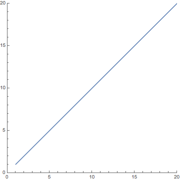
1. (20, 20), using the interval 0 ≤ t ≤ 4

   With these initial conditions you should have found that neither army gained the long term advantage. Your plot should have shown that the curve never actually even intersected an axis, and stabilized at a value of approximately (1,1). Even increasing the upper bound on t will make no difference to this end-result. This would translate into a prediction that in the long term the two armies will fight to a stalemate, both maintaining a size of about 10,000 troops each. Your graph should have looked something like this:

   
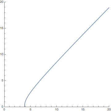
2. (21, 20), using the interval 0 ≤ t ≤ 1

   With these initial conditions you should have found that the British army won the battle, with the plot leaving the first quadrant at coordinates (3.871, 0). This would translate into a prediction that the British killed all of the opposing French army, and was left with approximately 38,710 of their own troops after the battle. Your graph should have looked something like this:

   
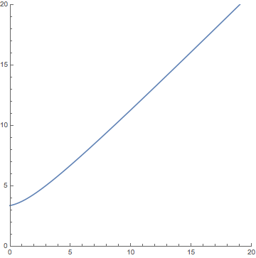
3. (20, 21), using the interval 0 ≤ t ≤ 1

   With these initial conditions you should have found that the French army won the battle, with the plot leaving the first quadrant at coordinates (0, 3.3803). This would translate into a prediction that the French killed all of the opposing British army, and was left with approximately 33,803 of their own troops after the battle. Your graph should have looked something like this:

   

Combining these three plots into a single graph would produce the following:

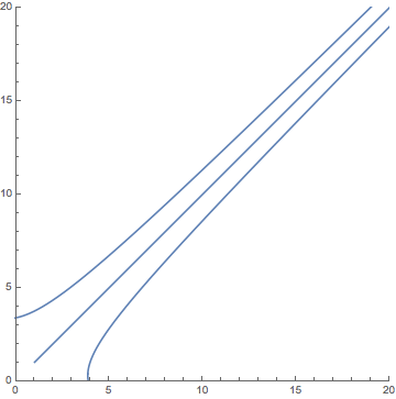
This image—a rudimentary phase-plane diagram of the model—reveals the that the initial condition (20, 20) that we used in our first analysis was somewhat special. Can you make a generalization about other initial conditions, based on what you observe in the above plot?

Well, that wraps up yet another lab. Let's return to the main table of contents page...

If you're lost, impatient, want an overview of this laboratory assignment, or maybe even all three, you can click on the compass button on the left to go to the table of contents for this laboratory assignment.