Numerical Methods - Euler Method
Numerical Methods for Solving Differential Equations
Euler's Method
Theoretical Introduction
Throughout this course we have repeatedly made use of the numerical differential equation solver packages built into our computer algebra system. Back when we first made use of this feature I promised that we would eventually discuss how these algorithms are actually implemented by a computer. The current laboratory is where I make good on that promise.
Until relatively recently, solving differential equations numerically meant coding the method into the computer yourself. Today there are numerous solvers available that can handle the majority of classes of initial value problems with little user intervention other than entering the actual problem. However, occasionally it still becomes necessary to do a some customized coding in order to attack a problem that the prewritten solvers can't quite handle.
This laboratory is intended to introduce you to the basic thinking processes underlying numerical methods for solving initial value problems. Sadly, it probably won't turn you into an expert programmer of numerical solver packages (unless some miracle occurs.)
The laboratory introduces you to a very simple technique for handling first order initial value problems. Like so many other concepts in mathematics, it is named after Leonhard Euler (1707-1783), perhaps the most prolific mathematician of all time. Before we can begin to describe Euler's Method, we must first make sure that we understand the nature of these approximate numerical solutions that his idea makes it possible for us to find.
The Nature of Numerical Solutions
From the point of view of a mathematician, the ideal form of the solution to an initial value problem would be a formula for the solution function. After all, if this formula is known, it is usually relatively easy to produce any other form of the solution you may desire, such as a graphical solution, or a numerical solution in the form of a table of values. You might say that a formulaic solution contains the recipes for these other types of solution within it. Unfortunately, as we have seen in our studies already, obtaining a formulaic solution is not always easy, and in many cases is absolutely impossible.
So we often have to "make do" with a numerical solution, i.e. a table of values consisting of points which lie along the solution's curve. This can be a perfectly usable form of the answer in many applied problems, but before we go too much further, let's make sure that we are aware of the shortcomings of this form of solution.
By it's very nature, a numerical solution to an initial value problem consists of a table of values which is finite in length. On the other hand, the true solution of the initial value problem is most likely a whole continuum of values, i.e. it consists of an infinite number of points. Obviously, the numerical solution is actually leaving out an infinite number of points. The question might arise, "With this many holes in it, is the solution good for anything at all?" To make this comparison a little clearer, let's look at a very simple specific example.
An Example
Say we were to solve the initial value problem:
y′ = 2x
y(0) = 0
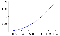
It's so simple, you could find a formulaic solution in your head, namely y = x2. On the other hand, say we were to use a numerical technique. (Yes, I know we don't know how to do this yet, but go with me on this for a second!) The resulting numerical solution would simply be a table of values. To get a better feel for the nature of these two types of solution, let's compare them side by side, along with the graphs we would get based on what we know about each one:
| Formulaic Solution | Numerical Solution | ||||||||||||||||||
|---|---|---|---|---|---|---|---|---|---|---|---|---|---|---|---|---|---|---|---|
| y = x2 |
|
||||||||||||||||||
 |
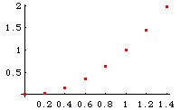 |
Notice that the graph derived from the formulaic solution is smoothly continuous, consisting of an infinite number of points on the interval shown. On the other hand, the graph based on the numerical solution consists of just a bare eight points, since the numerical method used apparently only found the value of the solution for x-increments of size 0.2.
Using Numerical Solutions
So what good is the numerical solution if it leaves out so much of the real answer? Well, we can respond to that question in several ways:
The numerical solution still looks like it is capturing the general trend of the "real" solution, as we can see when we look at the side-by-side graphs. This means that if we are seeking a qualitative view of the solution, we can still get it from the numerical solution, to some extent.
The numerical solution could even be "improved" by playing "join-the-dots" with the set of points it produces. In fact this is exactly what some solver packages, such as Mathematica, do do with these solutions. (Mathematica produces a join-the-dots function that it calls InterpolatingFunction.)
When actually using the solutions to differential equations, we often aren't so much concerned about the nature of the solution at all possible points. Think about it! Even when we are able to get formulaic solutions, a typical use we make of the formula is to substitute values of the independent variable into the formula in order to find the values of the solution at specific points. Did you hear that? Let me say it again: to find the values of the solution at specific points. This is exactly what we can still do with a numerical solution.
The Pitfalls of Numerical Solutions
One last word of warning, however, before we move on to actually finding numerical solutions. In a problem where a numerical solution would really be necessary, i.e. one which we can't solve by any other method, there is no formulaic solution for us to compare our answers with. This means that there is always an element of doubt about the data we produce by using these numerical techniques.
Say, for example, you obtained a set of numerical data as a solution, which led to the following graph:
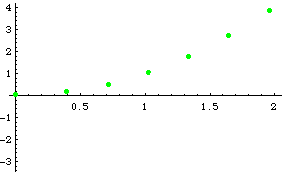
Any reasonable observer of this picture would, in the absence of any other evidence, assume that the underlying solution had a graph that looks something like this:
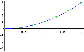
In other words, you'd play join-the-dots visually. But how do you know that the actual underlying solution doesn't look like this:
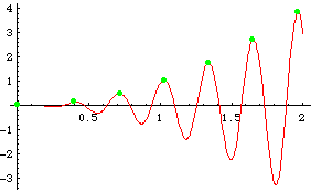
Notice that this graph fits the data points just as well as the first attempt we made at joining the dots, see:
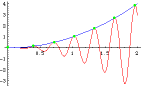
So how can you tell whether or not your data is leading you to the wrong conclusion? There are ways, both qualitative and quantitative, that can be used to help in making this kind of decision. A whole field of study called numerical analysis is dedicated to answering this sort of question. Suffice it to say, that in reality, the kind of error I've just illustrated with the above pictures never occurs. I deliberately used an "off-the-wall" example to get your attention.
In reality, the kind of errors we need to be careful of are much more subtle. What tends to happen with numerical solutions is that the calculated points drift further and further away from the actual solution as you move further and further from the point defined by the initial condition. This can lead you to make assumptions about the actual solution which aren't true.
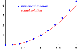
This difficulty can be overcome to some degree by calculating these points closer together. The penalty for this, of course, is that more points must be found, so the computer has to spend more time finding the solution. Most computer solvers try to strike a compromise between the accuracy inherent in using more points, and the extra time required to calculate the additional points. (A third issue involves machine round-off errors, but we won't even start to talk about that here.)
Now that we have been exposed a little to the type of solutions that we'll be finding, and the problems inherent in this kind of solution, it's time we found out how they can be generated.


